Introduction

Optimization of Indistinguishable
Two-Photon Absorption

Three-level system

We investigate the excitation of a three-level ladder-type atom by a unidirectional field containing a pair of indistinguishable photons. Starting from an analytical expression for the two-photon absorption probability, we determine the two-photon state that maximizes the population of the upper atomic state. We show that in the limit of an infinitely long pulse, perfect excitation is possible. The mathematically optimal state is identified as the time-reversed counterpart of the two-photon state emitted in spontaneous cascade decay.

We then compare this ideal excitation strategy with experimentally accessible families of states, analyzing how the optimal conditions depend on the ratio of atomic decay rates and on the separation of the atomic transition frequencies. Crucially, for indistinguishable photons described by Gaussian pulses, quantum interference may shift the maxima of the marginal spectral distribution away from the atomic resonances, qualitatively modifying the optimal excitation strategy.

The Core Model

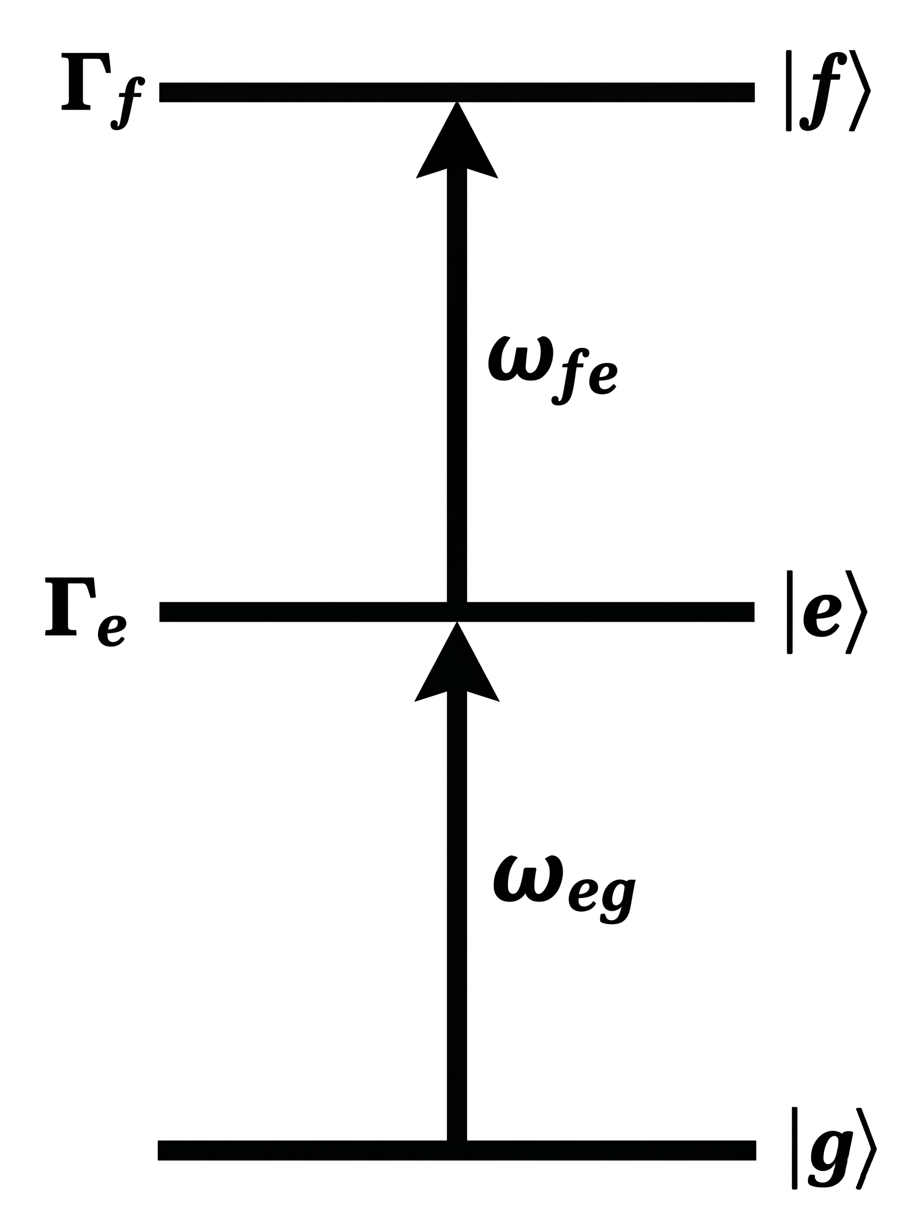
For the three-level system shown in the diagram, the probability of successful two-photon excitation at time \(t\) is:

Two-photon excitation probability Eq. (14) · p. 3
\[ P_{f}(t)= 4\Gamma_{e}\Gamma_{f}e^{-\Gamma_{f}t} \left|\int_{t_0}^{t}dt_2\, e^{\left(i\omega_{fe}+\frac{1}{2}(\Gamma_{f}-\Gamma_{e})\right)t_2} \int_{t_0}^{t_2}dt_1\, e^{\left(i\omega_{eg}+\frac{\Gamma_{e}}{2}\right)t_1} \Phi_{\rm sym}(t_1,t_2) \right|^2 \]

Here \(\Gamma_e\) and \(\Gamma_f\) are the decay rates of the intermediate and final states. The atomic transition frequencies are \(\omega_{eg}\) and \(\omega_{fe}\). Throughout the interactive sections, the atomic detuning is \(\delta_a = \omega_{fe} - \omega_{eg}\). Also \(\mu\) is the delay between the mean arrival time of the two photons. Three specific state architectures are studied: the optimal state and two variants of Gaussian states. Their mathematical definitions are presented within their respective interactive sections.

Note: This platform is a supplementary interactive guide. We highly encourage reading the main manuscript alongside this website to fully understand the theoretical derivations.

For our previous foundational work on distinguishable photons, please refer to: Phys. Rev. A. 111, 033709 (2025).

scroll to explore

Two-photon State Probability Distributions

For each photon-pair architecture, we compute the joint two-photon probability distribution \(p(t_1, t_2)\) and \(p(\omega_1, \omega_2)\) together with their marginals \(P(t)\) and \(P(\omega)\). The slider for \(\Gamma_e/\Gamma_f\) and \(\delta_a/\Gamma_f\) controls which parameter row is displayed. The checkbox toggles between optimised and fixed \(\delta_f\).

State I (Optimal) Eq. (19) · p. 4
\[ \Phi_{\rm opt}(t_1,t_2)= \frac{e^{\frac{1}{2}\Gamma_{f} t_2 -\frac{1}{2}\Gamma_{e}(t_2-t_{1}) -i\omega_{fe}t_2-i\omega_{eg}t_1}} {\sqrt{\mathcal{N}_{\rm opt}}} \,\Theta(t-t_2)\,\Theta(t_2-t_1)\,\Theta(t_1-t_0) \] \[ \text{where } \Theta(x) = \begin{cases} 1 & x \ge 0 \\ 0 & x < 0 \end{cases} \] \[ \text{With } t_0 \to -\infty, \text{ the normalization is simply } \mathcal{N}_{\rm opt} = \frac{1}{\Gamma_e \Gamma_f} \]
\[ \Phi(t_1,t_2)=\sqrt{\frac{\Omega_{+}\Omega_{-}}{2\pi}} \exp\!\left\{ -\frac{\Omega_{+}^2}{8}(t_1+t_2-\mu)^2 -\frac{\Omega_{-}^2}{8}\bigl(t_1-(t_2-\mu)\bigr)^2 -i\omega_{01}t_1-i\omega_{02}t_2 \right\} \] \[ \delta_f = \omega_{02} - \omega_{01} \]
\[ \Phi_{\rm sym}(t_1,t_2)= \frac{1}{2\sqrt{\mathcal{N}}} \bigl[\psi_{a}(t_1)\psi_{b}(t_2) +\psi_{b}(t_1)\psi_{a}(t_2)\bigr] \] \[ \text{where }\quad \psi_{a,b}(t)=\left(\frac{\Omega_{a,b}^2}{2\pi}\right)^{1/4}\exp\left[-\frac{\Omega_{a,b}^2}{4}(t-\mu_{a,b})^2-i\omega_{a,b}t\right] \] \[ \text{and} \quad \mathcal{N} = 1+\frac{2\Omega_a\Omega_b}{\Omega_a^2+\Omega_b^2} \exp\left[-\frac{\mu^2\Omega_a^2\Omega_b^2+4\delta_{f}^2}{2(\Omega_a^2+\Omega_b^2)}\right] \] \[ \delta_f = \omega_b - \omega_a \]
Loading datasets…

Peak Positions of the Marginal Frequency Distributions

The peak positions \(\omega_\text{peak}\) of the single-photon marginal distribution \(P(\omega)\) are plotted as functions of \(\Gamma_e/\Gamma_f\) for each state. Two peaks may emerge as the intermediate-state decay rate changes. Reference lines show the bare resonances \(\omega_{fe}\) and \(\omega_{eg}\).

State I (Optimal)— marginal distribution Eq. (27) · p. 5
\[ p(\omega)=\frac{\Gamma_{e}(\Gamma_{e}+\Gamma_{f})\!\left(\Gamma_{e}+\tfrac{1}{4}\Gamma_{f}\right) +\Gamma_{e}(\omega_{fe}-\omega_{eg})^2 +\Gamma_{f}(\omega-\omega_{eg})^2} {4\pi \left[(\omega-\omega_{eg})^2+\tfrac{\Gamma_{e}^2}{4}\right] \left[(\omega-\omega_{fe})^2+\tfrac{(\Gamma_{e}+\Gamma_{f})^2}{4}\right]} \]
State II — marginal distribution Eq. (44) · p. 9
\[ \begin{aligned} p(\omega) = \frac{1}{\sqrt{\pi(\Omega_{+}^2+\Omega_{-}^2)}\,\mathcal{N}} &\Biggl\{ \exp\!\left(-\frac{4(\omega-\omega_{01})^2}{\Omega_{+}^2+\Omega_{-}^2}\right) +\exp\!\left(-\frac{4(\omega-\omega_{02})^2}{\Omega_{+}^2+\Omega_{-}^2}\right) \\&\quad +2\exp\!\left(-\frac{4(\omega-\bar{\omega})^2}{\Omega_{+}^2+\Omega_{-}^2} -\Omega^2\mu^2 -\frac{\delta_f^2}{\Omega_{-}^2}\right) \cos\!\left[\frac{2\Omega_{-}^2\mu}{\Omega_{+}^2+\Omega_{-}^2}(\omega-\bar{\omega})\right] \Biggr\} \end{aligned} \] \[ \text{Where}\quad \bar{\omega} = \frac{1}{2}(\omega_{01}+\omega_{02}), \quad \Omega^2 = \frac{\Omega_{+}^2\Omega_{-}^2}{\Omega_{+}^2+\Omega_{-}^2} \] \[\delta_f = \omega_{02} - \omega_{01} \] \[\mathcal{N} =1+\exp\left(-\frac{\Omega_{-}^2\mu^2}{4}-\frac{\delta_{f}^2}{\Omega_-^2}\right) \]
State III — marginal distribution Eq. (37) · p. 6
\[ p(\omega)=\frac{1}{2\mathcal{N}} \left\{ \left|\tilde{\psi}_{a}(\omega)\right|^2 +\left|\tilde{\psi}_{b}(\omega)\right|^2 +2\,\mathrm{Re}\!\left(\tilde{\psi}_{a}^{*}(\omega)\,\tilde{\psi}_{b}(\omega)\,x\right) \right\} \] \[ x=\sqrt{\frac{2\Omega_a\Omega_b}{\Omega_a^2+\Omega_b^2}} \exp\!\left\{ -\frac{\Omega_a^2\Omega_b^2\mu^2+4\delta_f^2 -4i\delta_f(\mu_a\Omega_a^2+\mu_b\Omega_b^2)} {4(\Omega_a^2+\Omega_b^2)} \right\} \] \[ \tilde{\psi}_{a,b}(\omega)=\left(\frac{2}{\pi\Omega_{a,b}^2}\right)^{1/4}\exp\left[-\frac{(\omega-\omega_{a,b})^2}{\Omega_{a,b}^2}+i\mu_{a,b}(\omega-\omega_{a,b})\right] \]
Loading datasets…

Peak Position of the Optimum-State Marginal Distribution

A focused view of the optimum-state frequency marginal peak positions derived analytically from Eq. (33) of the draft. Root-finding of the derivative locates the extrema as a function of \(\Gamma_e/\Gamma_f\) for the selected detuning \(\delta_a/\Gamma_f\).

Marginal distribution of State I (optimal) Eq. (27) · p. 5
\[ p(\omega)=\frac{\Gamma_{e}(\Gamma_{e}+\Gamma_{f})\!\left(\Gamma_{e}+\tfrac{1}{4}\Gamma_{f}\right) +\Gamma_{e}(\omega_{fe}-\omega_{eg})^2 +\Gamma_{f}(\omega-\omega_{eg})^2} {4\pi \left[(\omega-\omega_{eg})^2+\tfrac{\Gamma_{e}^2}{4}\right] \left[(\omega-\omega_{fe})^2+\tfrac{(\Gamma_{e}+\Gamma_{f})^2}{4}\right]} \]
Loading dataset…

About the Authors

Masood Valipour1,2
Quantum optics, open quantum systems
Gniewomir Sarbicki1,2
Quantum information, entanglement theory
Karolina Słowik1,2
Quantum nanophotonics, light-matter interaction
Anita Dąbrowska3
Open quantum systems, quantum stochastics

1 Institute of Physics, Faculty of Physics, Astronomy and Informatics, Nicolaus Copernicus University, Grudziądzka 5/7, 87–100 Toruń, Poland

2 Institute of Advanced Studies, Nicolaus Copernicus University, Wileńska 4, 87–100 Toruń, Poland

3 Institute of Theoretical Physics and Astrophysics, Faculty of Mathematics, Physics and Informatics, University of Gdańsk, Wita Stwosza 57, 80–308 Gdańsk, Poland